

Data Mining Misconceptions #2: How Much Data ...
By Tim Graettinger
“How much data do I need for data mining?” In my experience, this is the most-frequently-asked of all frequently-asked questions about data mining. It makes sense that this is a concern – data is the raw material, the primary resource, for any data mining endeavor. Data can be difficult and expensive to collect, maintain, and distribute. And those activities are just the prerequisites for extracting any value from it via data mining and modeling.
The question of data quantity does not stand apart from data quality, sampling, and a host of related other issues. Entire books describe these aspects in great detail. My goal is more modest: to discuss the symptoms and the treatments for one of the most common misconceptions about data quantity for data mining – believing (or hoping) that plenty of data is available for model building when it really isn’t.
Working with Pat and Liam
Pat and Liam are long-time friends (and clients). Our first collaboration took place over ten years ago. At that time, they had a project that was in trouble. Pat and Liam had engaged a firm to build a direct marketing model that would indentify good candidates (individuals) to contact for an insurance product. The trouble was that the model performed well on the data used to build it, but its performance was terrible on other data held out for independent testing. A mutual friend introduced me to Pat and Liam, thinking that I might be able to help. Early in our initial conversation, Pat said, “We have tons of data, almost a million records from the first direct mail campaign.” My spider-sense[i] was tingling. I had some suspicions and asked, “What was the overall response rate for that campaign?” Liam told me that it was about 0.1%, or 1 in 1000. My suspicion was that they were data-limited, in an important way. As we’ll soon see, my suspicion was on target.
The Data Quantity Problem in a Nutshell
The Quantity-Action matrix in Table 1 below outlines four situations that can occur, based on:
- the quantity of data available (enough or not enough)
- the data mining action taken (do nothing or do something)
As evident from the table, two situations are not problems (doing nothing when sufficient data is not available, and doing something when sufficient data is available). Two situations are problematic, however:
- Doing nothing when sufficient data is available for data mining. This results in missed opportunities.
- Doing data mining (or more accurately, trying to do too much) with limited data. That's trouble. In the jargon of data mining, this situation is termed “overfitting”, and it is my focus in this article.
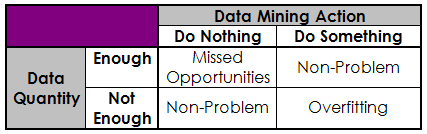 Table 1 - The Quanitity-Action Matrix
Detect, Diagnose, and then Prescribe...
Pat and Liam’s problem had the classic symptoms of overfitting – a model performs well on data used to build it, but poorly on data withheld for testing. As an analogy, think about custom-tailored clothes. They are cut very specifically for an individual, and they are unlikely to fit anyone else nearly as well, if at all. To understand how overfitting occurs in practice, we will use a greatly simplified example of data for a direct marketing model much like Pat and Liam’s. We will use my favorite, three-step approach to problem solving: detect, diagnose, and prescribe. In doing so, I will illustrate overfitting and how to correct it – so you can recognize and remedy it in your own work.
Step One: Detect
Good data mining practice requires splitting any data table into at least two segments[ii]. One segment is used to build, or “train”, the model. The other is a testing, or “hold out” segment that is used to validate the built model – checking the model’s performance and robustness on unseen or new data. For simplicity in our example, we will randomly select 50% of the data for training and 50% for testing.
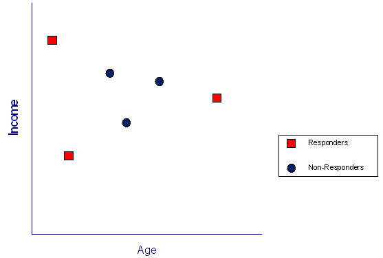
Figure 1 -Training data for the direct mail example
Figure 1 displays just the training data for our example. Red squares indicate persons who responded to a previous direct mail campaign, while the blue circles mark those who did not respond. For each person, we simply have information about their age and income. The goal of data mining will be to build a mathematical model to predict, based on age and income, which other people are most likely to respond to a future mailing.
We’ll use a mathematical model that separates responders from non-responders by means of straight lines. As shown in Figure 2, three lines do a very nice job of dividing the age-income landscape into responder and non-responder regions, designated by the red “R” and the blue “N”, respectively. Notice that the model makes no mistakes on the training data used to build it. Note also that two parameters – slope and intercept - define each of the separating lines. Three lines, then, require 6 parameters, which amounts to one per person in the training data.
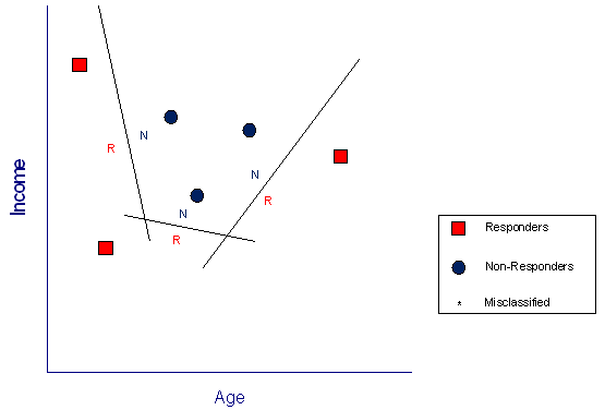
Figure 2 - Training data with straight lines separating responders and non-responders
Now comes the moment of truth – how does the model perform on the test data. In Figure 3, the model stays the same (that is, the position of the separating lines), but the data displayed is the testing data. The results are quite poor. Four of seven people are classified incorrectly (each is marked by an asterisk).
In our simple example, we detected a problem. How? Using good model-building practice, we separated the original data into a training set and a testing set. It is critical to detect the problem at this stage, before a model is put into service (for example, for a large-scale direct mail campaign). Because they did separate the data as described, Pat and Liam detected the problem with their model. They needed help with the next step, diagnosing the problem.
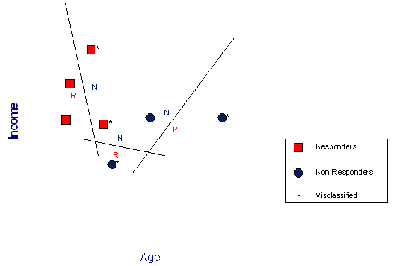
Figure 3 - Separating lines from the model applied to the testing data
Step Two: Diagnose
Diagnosing an overfitting problem requires two pieces of information:
- the number of records in the training set that belong to the minority group
- the number of parameters in the model
From these numbers we can compute the “fitting ratio”, FR, as:
FR = 2 x number of minority records / number of model parameters
In our simple example, we have 3 responders[iii]. As noted above, the number of parameters in our model is 6. Thus, the fitting ratio equation yields 2 × 3 ÷ 6 = 1.0 . Small fitting ratios (less than 10) are often red flags for overfitting. Small ratios mean that enough parameters (“handles”) may be available to dice up the landscape into pieces that can classify too precisely, or overfit, the training data.
Pat and Liam’s real-life model was a fairly complex, mathematical neural network consisting of about 2000 parameters. From my question about response rate, I could mentally estimate that the data set contained about 1000 responders. From these two numbers, I realized that their fitting ratio was close to 1.0 as well. So, despite the fact that their overall data set contained around a million records, the real limiting factor was the small number of responders. I was pretty sure about the problem, and the next step was to fix it.
Step Three: Prescribe
Usually, the best prescription for overfitting is conservative model-building. By conservative, I mean building simple models with few parameters – this is the portion of the fitting ratio that is easiest to impact[iv]. The resulting model is much more likely to perform similarly on training data and testing data. And this performance will be a much better indicator of the performance in actual use under real-world conditions.
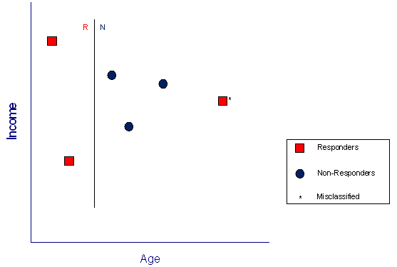
Figure 4 - New, simpler model built with the training data
For the example, I constructed a new, simpler model in Figure 4 that ignores income and simply classifies people based on age (thus, a one-parameter model, and a fitting ratio of 6). Note that the model misclassifies one person in the training data. When applied to the testing data in Figure 5, the new model also makes only a single error – now that’s more like it.

Figure 5 - New, simpler model applied to the testing data
A Happy Ending
A much more conservative model also solved the problem for Pat and Liam. By reducing the number of predictive factors (like age, income, etc.) and the complexity of the model, the fitting ratio was increased from 1.0 to about 100. The performance on testing data nearly equaled that on training data, and the model subsequently operated well when selecting prospects for the next mailing campaign.
The question of how much data you need for data mining is complicated. But here’s the good news: you can use what you’ve got, and then detect, diagnose, and prescribe when or if problems develop.
We would love to hear your comments or questions about this article. Drop Tim a note at tgraettinger@discoverycorpsinc.com, post a comment on our Journal page, or give us a call at (724)-743-3642.
Tim Graettinger, Ph.D., is the President of Discovery Corps, Inc., a Pittsburgh-area company specializing in data mining, visualization, and predictive analytics.
[i] Spider-Man is a comic book superhero. Like me, his spider-sense tingles when he senses trouble.
[ii] More sophisticated cross-validation schemes are often used in practice. But the train-test scheme with 50% of the data in each segment is useful for discussion.
[iii] Since we have equal numbers of responders and non-responders, we can choose either one as the minority group.
[iv] You can go out and get more data, too. That’s not always an easy option, but it should be considered.